Linear Regression
Introduction
Linear regression is a foundational concept in statistics and machine learning, serving as a fundamental technique for modelling the relationship between two or more variables. In this comprehensive article, we’ll delve into the intricacies of linear regression, covering its definition, mathematical representation, assumptions, types, and practical applications. Additionally, we’ll explore the process of fitting a linear regression line, including cost function optimization using gradient descent and evaluating model performance using the R-squared method.
Definition
Linear regression is a statistical method used to model the relationship between a dependent variable (target) and one or more independent variables (predictors) by fitting a linear equation to observed data.
Description
Linear regression aims to establish a linear relationship between the independent variables (X) and the dependent variable (Y) by estimating the coefficients (slope and intercept) of the linear equation. The model assumes that the relationship between the variables is linear, meaning that a change in one variable is associated with a proportional change in the other variable.
Assumptions
Linear regression relies on several assumptions, including:
- Linearity: The independent and dependent variables have a linear relationship with one another.
- Independence: The observations in the dataset are independent of each other.
- Homoscedasticity: The variance of the errors is constant across all levels of the independent variable.
- Normality: The errors are normally distributed around the regression line.
For Multiple Linear Regression, all four of the assumptions from Simple Linear Regression apply. In addition to this, below are few more:
- No Multicollinearity: This indicates that there is little or no correlation between the independent variables.
- Overfitting: Overfitting occurs when the model fits the training data too closely, capturing noise or random fluctuations that do not represent the true underlying relationship between variables. This can lead to poor generalization performance on new, unseen data.
Application
Linear regression is widely used in various fields, including:
- Economics: Predicting GDP growth based on factors like investment and consumption.
- Finance: Forecasting stock prices using historical data.
- Healthcare: Estimating patient outcomes based on clinical variables.
- Marketing: Predicting sales revenue based on advertising expenditure.
Types
Linear regression can be classified into two main types:
- Simple Linear Regression: Involves one independent variable.
- Multiple Linear Regression: Involves two or more independent variables.
Graphical and Mathematical Representation
Graphically, linear regression is represented by a straight line that best fits the observed data points.

Mathematically, the linear regression equation for -
1. Simple Linear Regression
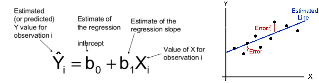
In simple linear regression, we have one independent variable X and one dependent variable Y. The relationship between X and Y is modelled using a linear equation with two parameters: the slope (β1) and the intercept (β0).
The equation for simple linear regression is given by:

where:
- Y is the dependent variable (target),
- X is the independent variable (predictor),
- β0 is the intercept (y-intercept),
- β1 is the slope (regression coefficient),
- ϵ is the error term.
2. Multiple Linear Regression
In multiple linear regression, we have multiple independent variables (X1,X2,…,Xn) and one dependent variable Y. The relationship between X and Y is modelled using a linear equation with n+1 parameters: one intercept (β0) and n regression coefficients (β1,β2,…,βn).
The equation for multiple linear regression is given by:
where:
- Y is the dependent variable (target),
- X1,X2,…,Xn are the independent variables (predictors),
- β0 is the intercept,
- β1,β2,…,βn are the regression coefficients,
- ϵ is the error term.
Linear Regression Line
The linear regression line is the line that best fits the observed data points, minimizing the sum of squared differences between the observed and predicted values. It is determined by estimating the coefficients θ0 and θ1 that minimize the residual sum of squares (RSS).
Finding Best Fit Line
- Cost Function: The cost function measures the difference between the predicted and actual values of the dependent variable. In linear regression, the most commonly used cost function is the Mean Squared Error (MSE), which calculates the average squared difference between the observed and predicted values.

Where hθ(x(i)) is the predicted value, y(i) is the actual value, and m is the number of observations.
- Gradient Descent: Gradient descent is an optimization algorithm used to minimize the cost function by iteratively updating the coefficients θ0 and θ1 in the direction of the steepest descent.


where α is the learning rate .

- Model Performance — R-squared Method: R-squared (R2) is a statistical measure that represents the proportion of the variance in the dependent variable that is explained by the independent variables in the model. It ranges from 0 to 1, with higher values indicating a better fit of the model to the data.

where:
- SSres is the sum of squared residuals (errors),
- SStot is the total sum of squares.
Conclusion
Linear regression is a powerful and versatile tool for modelling the relationship between variables in various fields. By understanding its principles, mathematical representation, assumptions, and techniques for model fitting and evaluation, practitioners can effectively apply linear regression to analyse data, make predictions, and derive valuable insights in real-world scenarios.
